More Hints for the Plugin Author

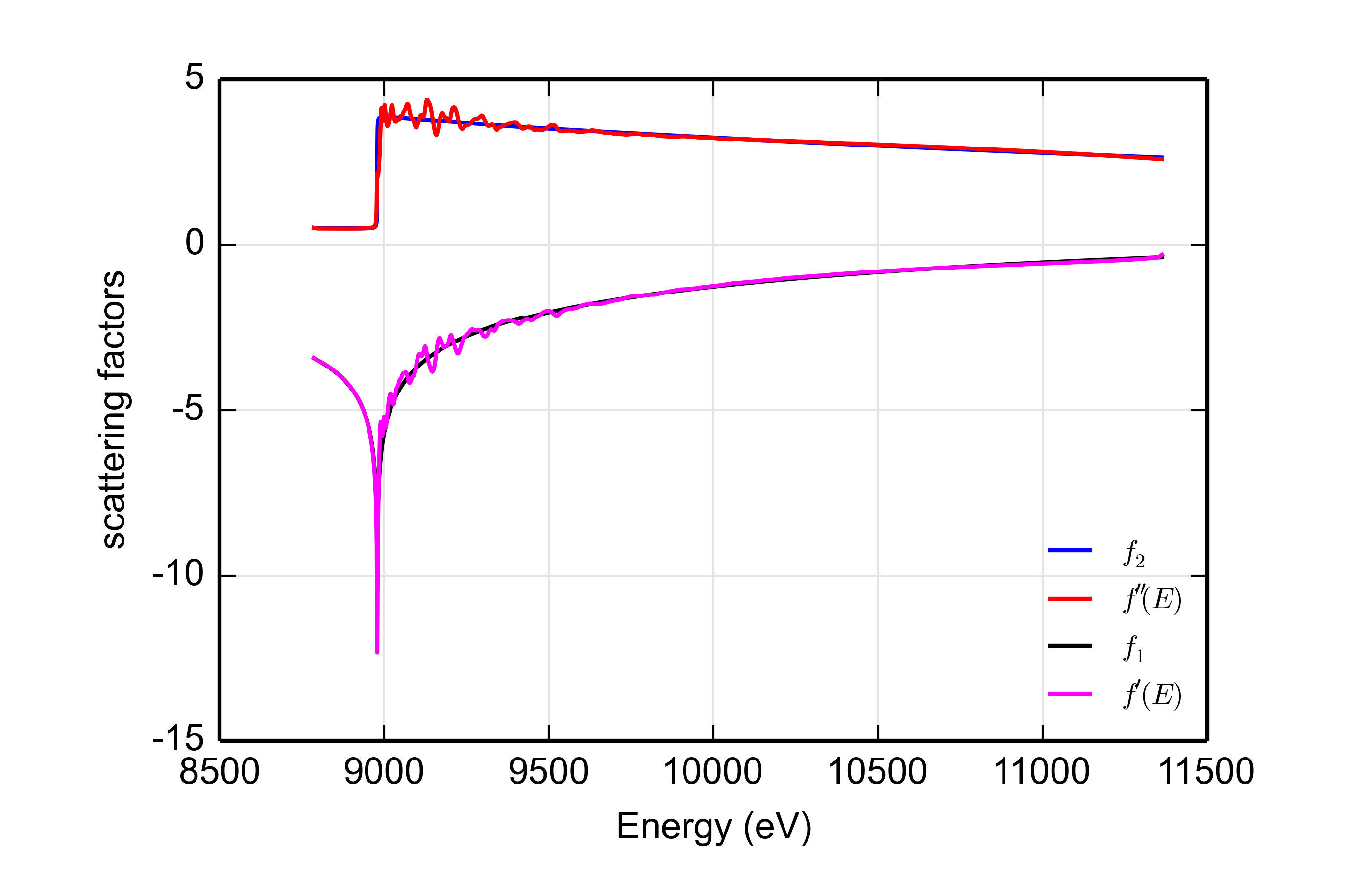
The diffKK plugin (at plugins/xafs/diffkk.py) implements the differential Kramers-Kronig transform suggested by Cross and Newville using the MacLaurin series algorithm suggested by Ohta and Ishida, Applied Spectroscopy 42:6 (1988) pp. 952-957. This is a way of matching experimental data to tabulated values of the imaginary part of the energy-dependent correction to the Thompson scattering factor and using a Kramers-Kronig transform to generate the real part. The advantage of this over the tabulated values is that, starting from a measured XAS spectrum, the diffkk results include the effect of the local scattering environment on the energy-dependent scattering function.

The diffKK plugin uses the MBACK plugin to do the matching of the XAS data to tabulated f​′′​​(E) data. It also demonstrates a few more features of Larch plugins that merit discussion in this tutorial.

A Larch plugin implementing a Group

The MBACK plugin implements one function, which is registered to Larch's symbol table. This function is intended for use with an existing data Group.

The diffKK plugin takes a slightly different approach. It too exposes a function in Larch's symbol table. This function is called diffkk and returns a reference to a diffKK Group. Here's what that looks like:

def diffkk(energy=None, mu=None, z=None, edge='K', mback_kws=None, _larch=None, **kws):
    """
    Make a diffKK group given mu(E) data

      Attributes
        energy:     energy array
        mu:         array with mu(E) data
        z:          Z number of absorber
        edge:       absorption edge, usually 'K' or 'L3'
        mback_kws:  arguments for the mback algorithm
    """
    return diffKKGroup(energy=energy, mu=mu, z=z, mback_kws=mback_kws, _larch=_larch)


def registerLarchPlugin(): # must have a function with this name!
    return ('_xafs', { 'diffkk': diffkk })

and here how it is called:

:FIXME: angle bracket wierdness

larch> dkk = diffkk(data.energy, data.xmu, z=29, edge='K', mback_kws={'e0':8979, 'order':4})
larch> show c
== diffKK Group: 7 symbols ==
  edge: 'K'
  energy: array<shape=(612,), type=dtype('float64')>
  kk: <bound method diffKKGroup.kk of <diffKK Group>>
  mback_kws: {'e0': 8979, 'order': 4}
  mu: array<shape=(612,), type=dtype('float64')>
  plotkk: <bound method diffKKGroup.plotkk of <diffKK Group>>
  z: 29

The diffkk function creates and returns a diffKK Group, which is called dkk. This Group contains the energy and μ(E) arrays, the scalar values of z and edge arguments, the dictionary value of the mback_kws argument, and references to a couple of functions, kk() and plotkk(). This really underscores the definition of a Group being a collection of things.

The diffKK Group is defined in the plugin as a class which inherits from Larch's Group. That is, diffKK has all the properties of a Larch Group and the additional properties given to it in this plugin.

class diffKKGroup(Group):
    """
    A Larch Group for generating f'(E) and f"(E) from a XAS measurement of mu(E).
    """

    def __init__(self, energy=None, mu=None, z=None, edge='K', mback_kws=None, _larch=None, **kws):
        kwargs = dict(name='diffKK')
        kwargs.update(kws)
        Group.__init__(self,  **kwargs)
        self.energy     = energy
        self.mu         = mu
        self.z          = z
        self.edge       = edge
        self.mback_kws  = mback_kws

        if _larch == None:
            self._larch   = Interpreter()
        else:
            self._larch = _larch

    def __repr__(self):
        return '<diffKK Group>'

In typical fashion, the class has a document string. The __init__ method of the class is defined and used to initialize various attributes of the class. Most of these attributes are the things that will be needed to perform the differential KK transform. It also defines a _larch reference which will point at the correct value of the Larch interpreter.

The __repr__ method is also specified so that the class has an unambiguous string representation:

larch> print dkk
<diffKK Group>

The plugin then goes on to define the kk() and plotkk() functions. Using the dkk group defined by the commmand above, you can perform the KK transform and plot the results. These commands post a plot to the screen:

larch> dkk.kk()
larch> dkk.plotkk()

The kk() function places additional arrays and scalars in the dkk Group.

This kind of plugin -- one which defines a Group and stores a tightly connected, curated collection of data and function references -- is very handy. It makes a nice, neat package for an analysis concept. See the section on Feff paths from the Larch document for several more examples of this sort of plugin.

Using NumPy effectively

The diffKK plugin also makes effective use of NumPy's vectorized calculations. At the heart of the diffKK algorithm is a computationally intensive KK transform. Here is a scalar implementation of the MacLaurin series algorithm

def kkmclr_sca(e, finp):
    """
    reverse (f''->f') kk transform, using maclaurin series algorithm
    """
    npts = len(e)
    fout = [0.0]*npts

    factor = -FOPI * (e[npts-1] - e[0]) / (npts - 1)
    nptsk  = npts / 2
    for i in range(npts):
        fout[i] = 0.0
        ei2 = e[i]*e[i]
        ioff = i%2 - 1
        for k in range(nptsk):
            j = k + k + ioff
            de2 = e[j]*e[j] - ei2
            if abs(de2) <= TINY:
                de2 = TINY
            fout[i] = fout[i] + e[j]*finp[j]/de2
        fout[i] *= factor
    return fout

(I have removed most of the document string and all of the exception handling for the sake of brevity.)

This has nested loops over the entire range of the arrays containing the data to be transformed. While the inner loops is smaller by a factor of 2 than the outer loop, this is effectively of order

(n​2​​) in calculation time. It scales poorly in time as the arrays become large.

Here is how this is implemented in diffKK:

def kkmclr(e, finp):
    """
    reverse (f''->f') kk transform, using maclaurin series algorithm
    """
    npts = len(e)
    fout   = np.zeros(npts)
    factor = -FOPI * (e[-1] - e[0]) / (npts-1)
    ei2    = e**2
    ioff   = np.mod(np.arange(npts), 2) - 1

    nptsk  = npts/2
    k      = np.arange(nptsk)
    for i in range(npts):
        j    = 2*k + ioff[i]
        de2  = e[j]**2 - ei2[i]
        fout[i] = sum(e[j]*finp[j]/de2)

    fout = fout * factor
    return fout

Here NumPy's vectorization is used to remove the inner loop. Calculations are made on entire vectors rather than by iterating over the elements of the inner loop. The iteration still happens, but it is done behind the scenes using NumPy's efficient vectorization. This is not quite as fast an order n calculation, but it is much faster than the scalar implementation above. On the modest and fairly old computer I am sitting at to write this, the scalar calculation takes about 15 seconds while the vectorized calculation takes under 2 seconds.

Take the time to understand how this vectorized math stuff works. It pays off!